Regression analysis is one of the most widely used statistical techniques. This method also forms the basis for many more advanced approaches. Ordinary Least Squares (or OLS) Regression brings insights into the dependencies of the variables and allows making predictions. But do we really understand the logic and the scope of this method? In this tutorial, we go through the basics of the OLS regression in R. As an example we will use a B2B logistics company dataset. For more in-depth counseling on data analysis within R you can always contact us for professional assistance – our experts are well-versed in all applications of statistical analysis in R!
Studying relationships with OLS regression in R
Scientists are often interested in understanding relationship between two (or more) concepts. Statistics provides the tools for studying such dependency by means of the OLS linear regression analysis. The starting point for this analysis, however, is always the scientist’s idea about the influence that one independent variable (X) has on another dependent variable (Y). In symbols this idea or hypothesis could look like this:
\(X \rightarrow Y\)This equation expresses that X is being impacted by Y. OLS linear regression analysis allows us to test the idea from a scientific viewpoint.
Example dataset: Do urgent orders predict total orders?
In this article we use the R statistical software for the analysis and an example Daily Demand Forecasting Orders dataset to illustrate our steps. The dataset can be downloaded as a .csv File and then imported into R with the following statement:
data<-read.csv("Daily_Demand_Forecasting_Orders.csv", head=TRUE, sep=";")
 dim(data)
The dataset includes 60 daily observations (i.e. rows of the table) of demand forecasting orders of a real Brazilian logistics company measured by 13 parameters (i.e. columns of the table). However, for the purposes of this OLS regression in R we concentrate only on two columns, or variables, namely:
- Urgent orders (amount)
- Total orders (amount)
We will analyze whether the amount of urgent orders has a significant impact on the amount of total orders. After all, urgent orders may require more resources and thus play a leading role in defining company’s total business capability. Furthermore, we will show how OLS linear regression can be used to predict the amount of total orders based on the available information.
OLS Regression in R: Visual representation and formula
The idea of OLS regression is most easily explained graphically. Let’s assume we are interested in how total orders are influenced by urgent orders.
Our two variables can be represented on axes of the 2D plot with the following R code:
attach(data)
 plot(x=Urgent.order, y=Target..Total.orders.,main="Urgent and Total Orders", xlab="Urgent orders", ylab="Total orders")
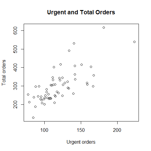
The points on the above plot are the real observations of the daily amounts of urgent and total orders. Each point in the graph represents one day in the 60-days observation period.
Visually there is a trend present: The higher the amount of urgent orders of the company, the higher the amount of its total orders. So far this seems logical. But unfortunately, our visual inspection does not count as a solid analytical tool. Hence, we use the analytical tools of the regression analysis in R to render further insights.
Inspecting possible linear relationships
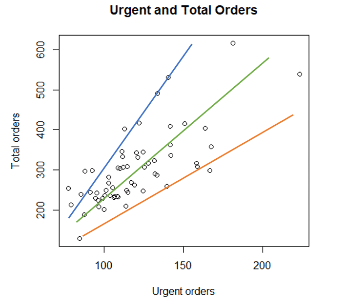
Urgent orders represent an independent variable, denoted as X. Total orders, on the other hand, are the dependent variable, denoted as Y. Let’s start by assuming the simplest form of interaction between X and Y, the linear one: Geometrically speaking, this relationship would form a straight line. It would mean that we can draw a line through the cloud of observations. But how shall we draw this line? One could think of many possibilities:
Findings the best line for OLS regression
Above we have seen 3 possible regression lines. But which one of these is the most suitable one for OLS regression?
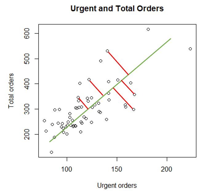
Intuitively it is clear that we want a line to lie as close to the observed points as possible. This is exactly the idea of the regression analysis. If we want the line be optimal, we want the distance (red spans in the picture below) between the line and the observation points to be minimal:
How is minimal distance determined?
So we want the distance to between the regression line and observed values to be minimal – but what distance is minimal?
One can say, the distance should be as close to zero as possible. But to check every little gap on the graph above does not sound very rational.
Alternatively, we could require the sum of distances to be minimal instead. However, some of those distances have a positive direction, while others have a negative direction. Therefore, summing up would lead to a score of almost zero even the gaps are large.
But luckily, statisticians found an elegant solution: We require the sum of squared distances, or mathematically put, the sum of squared residuals to be minimal. Denoting the residuals with e, we get the mathematical representation:
\(\sum_{i=1}^{n}=e_{i}^{2} \rightarrow min\)Because of this logic, the method is called the ordinary least squares estimation or OLS regression analysis.
As outlined above, the OLS regression is a standard statistical methods and is implemented in every statistical software. In R, there is the base function lm(), which performs the regression in R and computes the optimal regression line.
Prior to analyzing the R output, let us once again consider regression as a linear dependency. It is known that a line can be analytically formulated as:
\(y=\alpha +\beta \cdot x\)In our case, however, since the line only approximates the points but does not exactly go through them, we use a slightly different representation:
\(y=\alpha +\beta \cdot x+e\)This formula accounts for the error or residual term e. In these terms, α denotes the intercept point with the y-axis, and β stands for the slope of the regression line.
Involving R functionality: interpreting the output of the OLS regression in R
Below we outline the syntax to produce an output of the OLS regression in R.
The R function lm (linear model) is used, and the output with the relevant information is called by the summary function.
model_l<-lm(Target..Total.orders.~Urgent.order,data=data)
 Summary(model_l)
We will now go through the output step-by-step and interpret it.
OLS regression in R: The Call section

The first part of the output, “Call”, summarizes the model of the regression analysis in R. In our case it is a bivariate OLS regression, since we have only two variables: one dependent variable and one independent variable. Note that there can always be only one dependent variable (Y). Regression involving two or more independent variables (X) are called multiple OLS regression. These more advanced types of regression are outside the scope of this article.
OLS regression in R: The Residuals section

The next section, “Residuals”, contains the information on the residuals of the model. Here the residuals are summarized by descriptive statistics.
OLS regression in R: The Coefficients section

The most important information is contained in the section “Coefficients”. Here we see the least square estimators of both the intercept α and the slope β of our model. Slope is connected to the independent variable and can be therefore found in the “Urgent.order” row of the above table.
The results of the least square estimation appear in the “Estimate” column of the table. According to this, α = 14.676 and β = 2.407.
Interpretation of OLS regression coefficients
The intercept coefficient can be interpreted in the following way: It is the value of the dependent variable Y (total orders) when the independent variable X (urgent orders) is zero. In our case it would mean that without any urgent orders, the total amount of daily orders is around 14-15. However, the value of the intercept renders little practical use for our regression analysis in R.
Slope interpretation, in contrast, is always of utmost importance in the OLS regression analysis. The slope β coefficient shows how the dependent variable reacts to a change in the independent variable by one unit. Thus, if urgent orders increase by one, the amount of total orders would increase by 2,407. As we assumed in the beginning, this could happen because urgent orders require intensive resource allocation. This information is crucial for business planning purposes.
Other columns in the table contain standard error estimators and t-test statistics values. The t-test is used to check the following hypothesis:
H0: The independent variable has no significant effect on y
H1: The independent variable has a significant effect on y
Decision on the hypothesis is made based on the p-value in the last column of the table, “Pr(>|t|)”. If the p-value is smaller than the error probability, usually set to 5% or 0,05, then we can reject the null hypothesis and accept the alternative. In our case we conclude that urgent offers do have a significant effect on total offers, since the p-value is 0,0000000000372.
OLS regression in R: The Model section

The latter part of the output deals with an overall performance of the OLS regression model. Here we see the R-squared measure, describing the percentage of the total variance explained by the model. The highest possible value of R-squared is 1, meaning that the model explains 100% of the real dependencies. The lowest possible value of R-squared is 0, meaning that the model is practically useless. Output includes both multiple R-squared and adjusted R-squared measures. However, for the bivariate regression analysis in R both measures are suitable to access the model performance. In our case the model uncovers about 52% of the total variance or information, which is not a bad result.
Another important information is provided by the F-test. Contrary to the t-test, this test does not concern a single variable or coefficient, but the model as whole is tested:
H0: No one variable has no significant effect on y. In other words, the model provides no additional information.
H1: At least one variable has a significant effect on y. In other words, the model provides significant insights into the real-life dependencies.
The decision rule here (and in any other statistical test) is the same one as above for the t-test: If the p-value is smaller than 0,05, we can reject the null hypothesis and accept the alternative, and vice versa. In our case the F-test statistics is 66,09 with 1,58 df = degrees of freedom with p-value=0,00000000003719. This means that the model is statistically significant.
To sum up, we could conclude that amount of urgent orders of the logistics company does have a statistically significant positive effect on its total orders amount. We have reached this conclusion by means of the bivariate OLS regression analysis in R.
Did we do everything correct? Diagnostics of the OLS regression in R
After the regression in R is completed, one may ask if the model is justifiable from a mathematical standpoint. Like any other theory, OLS regression analysis is based on several assumptions, namely:
- Linearity: y depends on x by means of linear dependency
- Independence: Observation points \((x_{i} , y_{i})\) are independent of each other, meaning that the residuals are also independent
- Normality: The residuals e are normally distributed
- Homoscedasticity: Probably the least intuitively clear assumption. This means that variance of the residuals stays constant throughout the whole regression dataset.
How to check OLS regression assumptions in R with the plot() function
There are different methods and even readily available packages to test the assumptions of OLS in R. In this article we will consider one of these options with the built-in function for regression in R, plot():
par(mfrow=c(2,2))
 plot(model_l)
The first command is used to change the visual output and allow four plots to be displayed at once:
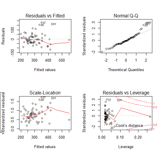
The first plot, “Residuals vs. Fitted” is helpful for the assessment of Linearity and Homoscedasticity: Linearity is met if the residuals (points on the plot) are mostly distributed around the zero line. Homoscedasticity means that there is no visible pattern of the residuals. This is sometimes referred to a distribution of residuals like “stars in the night sky”. As a further diagnostic tool one may apply the Breusch-Pagan homoscedasticity test. However, this is out of scope of this introductive tutorial. For an in-depth statistical consulting of OLS regression you can contact our experts at any time!
The second plot or QQ-plot is used to test the assumption of normality: the closer the residuals points are to the dotted 45 degrees line, the more likely the normality assumption is met. As we can see this is mostly the case for the observed values.
The third plot is also useful for checking the assumption of homoscedasticity: As in the first graph, we want to see no particular pattern in the residuals here.
Based on the above considerations one may conclude that the assumptions of the bivariate regression in R are met. We can therefore consider the results of the least squares estimation significant.
For further and more detailed analysis of the assumptions of the regression analysis in R you may always involve Novustat professional statistical analysis services.
What does the future hold: Predictions with the OLS Model in R
One of the most exciting functionalities of the regression analysis in R is its possibility to predict values of the dependent variable Y given the values of the independent variable X.
In our present example, we may want to predict the amount of total orders of our logistics company if urgent orders account for 100 items. In order to do so, first we need to define a new data set with these values:

Then, using the built-in function predict(), we obtain the corresponding total orders values under the 95% level of significance:

Therefore, we can estimate that if urgent orders constitute 100 items, total orders will account for 255 items. The predict() function also allows building prediction/confidence intervals and includes other forecasting options that are not included in our introduction tutorial.
Going further: possible variations and expansions of the OLS Model in R
This tutorial showed the basic functionality of the OLS regression in R. In addition, we also explained the statistical and mathematical logic behind this approach.
We used a simple example of the bivariate regression analysis in R. However, it is often beneficiary to include more than one predictor (independent variable X) into the model. This way one can often increase the model’s goodness-of-fit and prediction power.
We have, however, touched upon all the most important topics when performing regression analysis in R. Novustat experts are happy to support you and provide statistical counseling with further specific inquiries on the subject.
